INTRODUCTION
At present, Colombia is the second flower exporter in the world and the first in the Americas. According to reports given by the Flower and Foliage Chain of the Ministry of Agriculture and Rural Development (MADR) for the year 2017, there were 8.004 hectares dedicated to the production of ornamentals, an area that is distributed in the departments of Cundinamarca and Antioquia. The estimated annual total stem production is 242.944 t. This productive sector contributes significant economic income to the agricultural GDP, generating an income of foreign currency close to 1.312.000.000 US dollars, with roses contributing US$ 6,9 per exported kg yielding a 30% volume of the total exported stems.
The national production of flowers is made in a high percentage under greenhouse; the predominant structure is the traditional greenhouse that occupies 70% of the total area. Other types of greenhouse, such as the hanging greenhouse type, occupy the remaining 30%.
Temperature is one of the most relevant factors when programming climate control activities (Campen & Bot, 2001). Mainly because when it reaches extreme values in passive greenhouses (naturally ventilated) production is partially or totally limited (Kittas et al., 2005). The control of the temperature in the Colombian passive greenhouses is relevant in hot days of high radiation in which it is necessary to evacuate the thermal excesses produced in the interior. Under these conditions it is possible to reach temperatures close to 35°C according to Bojacá et al. (2009) and cause physiological disorders in plants (Sato et al., 2001). Additionally, these periods of high radiation usually generate dry and clear night conditions that favor the appearance of the phenomenon of thermal inversion, a phenomenon in which the interior temperature of the greenhouse is lower than that of the surrounding external air.
The study of the thermal and aerodynamic behavior of a greenhouse can be done through empirical models of energy balance, field experimentation, digital thermography or through numerical simulation applying techniques such as computational fluid dynamics (CFD) (Chen, 2009). This tool allows the qualitative and quantitative analysis of the thermal behavior of agricultural or livestock structures under different simulation scenarios (Norton et al., 2007).
The objective of this work consisted in developing and adjusting a 3D CFD numerical model, in order to study the thermal behavior of a Colombian hanging greenhouse under climatic conditions of the Bogotá savanna used for the production of rose (Rosa sp.).
METHODS
Site and Greenhouse Description
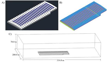
The experimental work was developed in a greenhouse with 8640 m2 of covered area, belonging to a farm dedicated to cut rose production (5º03'22.16''N, 73º55'49.07''W, 2583 masl) located in Cogua Municipality (Cundinamarca). The evaluated greenhouse consisted of 24 spans each with a width of 6.0 m (Figure 1A), the minimum and maximum heights under the channel were 3.2 and 6.4 m, respectively. The longitudinal distance of the greenhouse was 60 m and was oriented in the northeast-southwest direction (NE-SW). Each span had a moveable roof ventilation opening 1.0 m wide and 48 m long and fixed lateral openings 1.9 m wide on each of the four sides of the structure, for a total natural ventilation area of 1927 m2.
The exterior meteorological conditions were evaluated for 24 hours a day, within the period between 00:00 hours on March 29 and 23:00 hours on May 2, 2016. The variables were recorded through of a weather station (Vantage Pro2 Plus, Davis Instruments, Hayward CA), which integrated sensors for global radiation, temperature, relative humidity, precipitation, wind speed and direction with a registration frequency of 10 minutes.

FIGURE 1.
A) Isometric view of the evaluated greenhouse, B) mesh detail y C) computational domain.
Numeric Simulation
The CFD numerical simulation allows solving the governing equations of fluid flow using the finite volume method (Molina et al., 2009). These equations can be represented as convection-diffusion equations of a fluid for three conservation laws, which include the moment, energy and transport equations of a compressible fluid and in a three-dimensional (3D) field and are expressed as follows:
where ρ is the fluid density (kg m-3), ∇ is the nabla operator, φ represents the concentration variable, is the velocity vector (m s-1), Γ is the diffusion coefficient (m2 s-1) and S represents the source term (Piscia et al., 2012). The turbulent nature of the airflow was simulated using the standard turbulence model k-ε, which is based on two main equations, one for k representing kinetic energy and the other for ε representing the rate of dissipation in time and volume units. The transport equations for k and ε can be modeled as:
where μ is the viscosity and is turbulent viscosity in (kg m-1s-1), are the turbulent Prandtl numbers of Prandtl for k and ε. G k is the generation of turbulent kinetic energy due to velocity gradients, G b is the generation of turbulent kinetic energy due to buoyancy, Y M is the fluctuating dilation in turbulence due to the global dissipation rate and v is the kinematic viscosity coefficient. C 1ε , C 2ε , C μ , σ k and σ ε are constants with default values. This standard model k-ε has been widely used and validated in studies focused on greenhouses demonstrating an adequate precision (Fatnassi et al., 2006; Katsoulas et al., 2006). All the simulations considered the energy equation, which allowed analyzing the scalar field of temperatures inside the greenhouse. Likewise, the phenomenon of buoyancy was modeled. A phenomenon that drives the movement of air under the condition of external speed was made by means of the Boussinesq approach, which is described as follows:
where ρ ref is the constant density of the flow; T ref is the actual temperature (°C) and β is the coefficient of thermal expansion for air (β = 0.00329°C-1). The Boussinesq approximation is valid if the temperature differences that appear in the computational domain are not too large β(T-T ref ) < 1, a situation that generally occurs in the microclimate study of greenhouse (Baeza et al., 2006).
The selected radiation model was that of discrete ordinates (DO) with angular discretization. This model allows the analysis of climate under nighttime conditions, simulating and resolving the radiation phenomenon from the greenhouse floor to the external environment. For this purpose, the sky was considered a black body with an equivalent temperature (T C ) of 0°C for a predominant scenario of wet and clear nights (Iglesias et al., 2009).
Computational Domain and Mesh Generation
The ANSYS ICEM CFD preprocessing software (v. 17.0) was used to generate a large computational domain composed of the greenhouse and its surroundings. In order to guarantee the no affectation of the numerical solution of the flow field outside the greenhouse and to allow an appropriate definition of the atmospheric boundary layer (Rico, 2011) The dimensions of the computational domain were 354, 260 and 70 m for the x, y and z axes, respectively (Figure 1C). This size was determined following the guidelines for calculating the wind environment around the buildings using CFD (Tominaga et al., 2008). The computational domain consisted of an unstructured mesh of 76.651.871 volumes discretized in space, this number of elements was obtained after verifying the independence of the numerical solutions of the airflow at mesh sizes with a higher and lower number of elements according to the procedure reported by He et al. (2017). A fundamental criterion to establish the accuracy of the solutions is to evaluate the quality of the mesh (Figure 1B). The quality parameters evaluated were the cell size and the cell-to-cell size variation, finding that 93,1% of the cells in the mesh were within the high-quality range (0,95-1). The orthogonal quality was also evaluated, where the minimum value obtained was 0.94, results that were classified within the high-quality range (Flores et al., 2015). The convergence criteria of the model were established in 10-8 for the energy equation and 10-6 for the continuity, momentum and turbulence equations (Baxevanou et al., 2017).
Boundary Conditions
The upper limit of the domain and the surfaces parallel to the flow were set with boundary conditions of symmetrical properties so as not to generate frictional losses of the airflow in contact with these surfaces. The simulations considered the atmospheric characteristics of Cogua Municipality such as atmospheric pressure of 74992 Pa, air viscosity equal to 1,7E-05 kg m-1 s-1 and gravity of 9.81 m s-2. Other properties for polyethylene and agricultural soil such as specific heat (Cp), thermal conductivity (k) and density (ρ) were established according to Villagrán et al. (2012). The perimeter boundaries of the computational domain were established as limits of air intake or pressure output as the case may be. A uniform profile of wind speed was considered, evaluating speeds with values between 0.001 and 1.21 m s-1 and average temperature values for each hour of the day. These values were established based on the climatic information collected during the experimental measurement period.
Other input parameters that are necessary to feed the radiation model are the optical properties of the roofing material such as, absorption coefficient (α) of 0,69, transmission coefficient (Ƭ) of 0,19 and reflection coefficient (ρ) of 0,11. The model did not include any crop and a maximum hermetic seali ng of the greenhouse was assumed. These simplifications are valid since they are applied to each of the simulated cases and the errors that may arise will have the same degree of magnitude for each scenario.
Considered Scenarios
The evaluation was carried out assuming the average meteorological conditions for each hour evaluated (Table 1) and the standard ventilation configuration of the greenhouse studied, which, for this case, was lateral ventilation combined with roof ventilation for daytime hours (6-18 hours) and roof ventilation for nighttime conditions (19-5 hours).
TABLE 1.
Average meteorological conditions used as input parameters to the CFD-3D model
Model Validation
The validation of the CFD model was made through the comparison between the results of the simulations and the experimental records for the same temporal frequency of the temperature inside the real greenhouse during the evaluation period. The temperature of the greenhouse air was recorded by means of thirty T-type thermocouples (copper-constantan) connected to an equal number of data recorders (Cox-Tracer Junior, Escort DLS, Edison, NJ) deployed uniformly at 1,5 m from the ground surface and recording data every 10 minutes.
RESULTS AND DISCUSSION
Model Validation
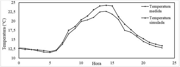
The model validation was made by comparing the temperature values measured experimentally and those obtained through CFD simulations, for the 24 hours of the day. Figure 2 shows the behavior of the temperature for each evaluated hour, showing a good fit between the two methodologies used and the same trend for the measurement period. Quantitatively, when comparing the measured and simulated data, an average absolute percentage error (MAPE) of 4,26% was obtained, an absolute mean error (MAE) of 0,75°C and a mean square error (MSE) of 0,94°C, values that guarantee that the use of the CFD model is adequate for the evaluation and description of the thermal behavior of the greenhouse.
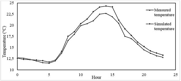
FIGURE 2.
Temperature profile measured and simulated inside hanging greenhouse type.
Daytime Period
Table 2 shows the time evolution of the interior greenhouse temperature for the daytime period. It is observed that the variable presented a minimum value of 12,17°C for hour 6 and reached a maximum value of 24,31°C at hour 14, this temporary increase is driven by the solar radiation. The thermal difference between the interior and the exterior of the greenhouse (ΔT = T internal -T external ) exhibited a minimum value of 0,88°C for the hour 6. This value is consistent since the indoor air comes from an energy loss process during the night hours and additionally, the solar radiation for the hour 6 is generally low in the intertropical zones, therefore, the energy gain inside the greenhouse is also low. The maximum value of ΔT was 5,93°C for hour 14, a value that is generated as a function of the thermal gain inside the greenhouse over the course of 7 hours (7-14 hours).
TABLE 2.
Average interior temperature and thermal difference between the interior and exterior of the greenhouse for simulated daytime scenarios
Temperature is one of the main parameters that affects the quality and growth of the flower stems. In the case of rose cultivation, it is recommended that optimum temperatures during the daytime period should be between 21 and 24°C Yong (2004). For the evaluated case, it is observed that this is fulfilled for the period between 11 and 16 hours; however, for the remaining hours the temperature are lower than recommended; this translates into longer vegetative cycles and lower stem production (Zieslin and Mor, 1990). Additionally, temperatures between 15 and 20°C under high humidity conditions favor the germination of Botrytis cinerea conidia (Restrepo, 2010), a disease that generates great economic losses for rose crops in the Bogota savanna.
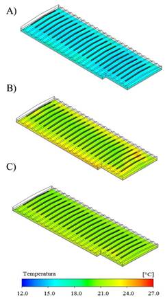
Figure 3 shows the thermal distribution patterns in a greenhouse section at 1.5 m from ground level for the hours 8, 12 and 16 (Figure 3 A-C). For the eight hour, a homogeneous thermal behavior can be observed with an average value of 17,52°C (Figure 3A). For the twelfth hour an average temperature of 23,05°C was obtained, under this condition a heterogeneous behavior was observed in 40% of the evaluated area. Higher temperatures were found near the lateral zones with averages of 25,1°C and lower temperatures of 21,1°C in the central zone of the greenhouse, just in the areas of influence of the roof vents (Figure 3B). These heterogeneous conditions are not suitable for the production of flowers since they generate differentiated production volumes of stems in quantity and quality. For the sixteenth hour, the average interior temperature was 21,17°C, observing some areas with temperature values of 22,8°C near the lateral and frontal ventilation openings (Figure 3C). This allows us to conclude that the thermal conditions inside the greenhouse are not thoroughly homogeneous and the thermal behavior for the first hours of the day period are the most unfavorable for the production of roses.
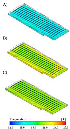
FIGURE 3.
Simulated temperature contours (°C) for A) hour 8, B) hour 12 and C) hour 16.
Night Period
Table 3 shows the average temperature values calculated for the night hours. The maximum temperature value of 16,19°C was registered for the hour 19, moment from which the behavior is decreasing as night passes. This is mainly due to the fact that under passive greenhouses an irradiative cooling is generated from the ground towards the external environment promoted by the confinement of the internal air and the high transmission of the plastic cover of the infrared radiation (Majdoubi et al., 2016).
The greenhouse has an acceptable thermal hermetic sealing, which allowed the generation of a positive ΔT for the hours evaluated, showing maximum and minimum ΔT values of 1,84 and 0,37°C for the first and last hour of the night, respectively. Taking into account that the general conditions were clear and humid it should be mentioned that the greenhouse presented a thermal behavior that limited the occurrence of the thermal inversion phenomenon that under these prevailing meteorological conditions is frequent within Colombian greenhouses.
The general recommendation for the cultivation of rose is to be able to guarantee night temperatures that oscillate between 15 and 17°C (Yong, 2004).The analysis of the data indicated that these recommended values are only obtained for hours 19 and 20. The following hours presented average values below the recommended value which can generate relevant effects on the growth and development of the plant; in productive terms, under these conditions it can be usual to obtain deformed flowers with a number of undesirable petals (Yong, 2004).
TABLE 3.
Average interior temperature and thermal difference between the interior and exterior of the greenhouse for simulated nighttime scenarios
| Hour | Average internal temperature (°C) | Thermal difference (ΔT, °C) |
|---|---|---|
| 19 | 16,19 | 1,84 |
| 20 | 15,23 | 1,73 |
| 21 | 14,25 | 1,27 |
| 22 | 13,76 | 1,17 |
| 23 | 13,29 | 1,04 |
| 0 | 12,62 | 0,78 |
| 1 | 12,34 | 0,60 |
| 2 | 12,29 | 0,72 |
| 3 | 12,19 | 0,75 |
| 4 | 12,06 | 0,74 |
| 5 | 11,76 | 0,37 |
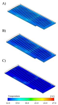
The qualitative analysis of thermal distribution patterns in a horizontal plane at 1.5 m above ground level for hours 20, 0 and 4 is presented in Figures 4 A, B and C. In general, a homogeneous thermal behavior is observed for the three hours evaluated in approximately 95% of the evaluated area.
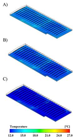
FIGURE 4.
Simulated temperature contours (°C) for A) hour 20, B) hour 0 and C) hour 4.
CONCLUSIONS
A 3D CFD model was generated to study the thermal behavior of a Colombian-hanging greenhouse. The model was validated through the comparison of experimentally obtained data and simulated data. This comparison showed an adequate degree of adjustment and the same trend, which allows concluding that the CFD model is reliable to develop numerical simulations and can be used to evaluate the thermal behavior of another type of greenhouse under the same meteorological conditions.
The results showed an optimal thermal behavior for six of the thirteen hours evaluated during the daytime period, during these six hours the temperature ranged in the optimum interval for the production of rose that is between 21 and 24°C. For the night period it was found that the thermal behavior is inadequate for nine of the eleven hours evaluated, the temperature values were lower than the recommended minimum of 15°C. These conditions can limit the final production of the rose crop and the commercial quality of the flower stems.
It is recommended that subsequent studies include another series of climatic parameters, such as relative humidity, vapor pressure deficit or ventilation rates, which will allow an analysis of the microclimatic behavior of the greenhouse and relate it to the agronomic and physiological behavior of the plants.

