ORIGINAL ARTICLE


http://opn.to/a/bFWi2

Methodology for Estimating Furrow Inflow Rate by Means of Chezy and Bazin’s Equations


ABSTRACT

The investigation was developed in the Basic Unit of Cooperative Production Albio Hernández of the Sugar Company Primero de Enero of the Ciego de Avila Province. The results demonstrated that the geometric parameters of the furrow in the sugar cane cultivation reached average values of 0.159 m; 0.590 m; 0.032 m and 1.756 m for the maximum height, the top width, the bottom width and the side slope coeficient, respectively. The simple potential model type y=eT f allows estimating in reliable way the water depth of circulation in the furrow starting from the direct mediation of the top width in the furrow. The values of the µ and ξ coefficients oscillate from 4.08 to 5.45 and 0.51 to 0.62, respectively and they are of great utility for the calculation of the cross sectional area and the hydraulic area of the furrow. The proposed methodology demonstrated, through the Average Percentage Error, its high accuracy to estimate the flow applied in the opening of the furrow.

Keywords: 

Ruggedness coefficient; hydraulic of furrows irrigation; speed of the water.


INTRODUCTION

Surface irrigation is the most used system, occupying the immense majority of the lands of irrigable at world level (Sánchez et al., 2002). Superficial irrigation in Cuba occupies 71% of the irrigated total area and it is in a critical technological state due to the absence of improvement investments (Pérez et al., 2013).

Superficial irrigation is intrinsically less efficient than the aspersion and the drip, because losses for deep percolation and runoff are inevitable (Génova et al., 2014); but the design and appropriate management allows the efficient and uniform irrigation of the lot (Faci & Playán, 1996; González & Playán, 1996).

In many countries of the world, the investigations are carried out with the purpose of replacing the furrows irrigation for pressure methods; however, the economic-financial situation of the producers restricts in many occasions the possibility of carrying out this technological exchange rate. Hence, the potential alternative is the superficial irrigation (Durán & García, 2007).

The knowledge of the relationship between soil type, water and cultivation allows the application of water in convenient quantities, according to the irrigation system to be used. That is why water measuring is essential for the maximum use of the resource Carrión (2015). On the other hand, it is necessary that the farmer familiarizes with the terms associated with the mensuration of the inflow rate (Bello & Pino, 2000).

Irrigation design consists on determining the optimal inflow rate and the time during which this flow is applied in the head of the field to achieve the biggest possible uniformity of application, for a longitude and a particular soil type (Saucedo et al., 2013). The objective of the present work consists on evaluating a methodology proposed to estimate the furrow inflow rate from Chezy and Bazin’s Equations.

MATERIALS AND METHODS

The investigation was developed in a lot of sugar cane of the variety C-120 located in the block 609 of the Basic Unit of Cooperative Production (UBPC) Albio Hernández of Primero de Enero Sugar Company, in Ciego de Ávila province. The irrigation system used is the type furrows irrigation, by means of pipes with multiple floodgates formed by a buried pipe of PVC with diameter of 315 mm that goes out directly of the station of pumping with a maximum longitude of 500 m in which the valves that supply water to the irrigation pipes of PVC with diameter of 280 mm are placed. This has adjustable floodgates every 1.50 m for the discharge of the furrow inflow.

Maximum height of the furrow (y max ), maximum top width (T max ) and bottom (b) were measured under experimental conditions in nine furrows selected at random inside the study area; later the furrow side slope coeficient was obtained by means of the following equation:

Furrow inflow rate was measured to the exit of the floodgates by means of the volumetric method; then, they were measured the times in which, the front of advance of the water flow, reached the stakes placed every 20 meters on the total furrow length of 100 m and average slope of 4.0‰. A digital chronometer of one-second accuracy was used. In these points, the value of top width (T i ) and flow depth (y i ) that allowed finding an adjustment model to estimate the flow depth in function of the top width of the water, were also obtained.

Validation of the statistical models was carried out by means of the Coefficient of Determination (R 2 ) according to Vicente et al. (2003) and the Half Percentage Error (Zúñiga & Jordán, 2005), with series of different data used properly for the generation of the model and the prediction. The equation used was the following:

Where APE is the Average Percentage Error (%); n the number of data of the series; y obs the observed variable; y sim the predicted variable.

The methodology proposed in this investigation is composed of the six following fundamental procedures. (1) Practical determination of the side slope coeficient of the irrigation furrows. (2) Determination of model that relates flow depth with the top width of the water in the furrow. (3) Obtaining of the coefficients μ and ξ to estimate the cross sectional area of flow, the wetted perimeter and the hydraulic radius of the furrow. (4) Estimating the speed of the water in the furrow irrigation according to the equation of Chezy and the coefficient of speed for the equation of Bazin. (5) Calculation of the furrow inflow rate by means of the equation of continuity. (6) Validation of the methodology proposed through the comparison between the furrow inflow rate real applied and the predicted ones.

RESULTS AND DISCUSSION

Analysis of Side Slope Coeficient in the Irrigation Furrows

Table 1 shows the values of geometric parameters of the furrow obtained directly in the different samplings points established in the experimental area. In Table 2, the main statistics corresponding to the descriptive analysis are shown. There, the mean values of the maximum height, maximum top width, bottom, and side slope were 0.159 m; 0.590 m; 0.032 m and 1.756, respectively, for what they should be taken as definitive design parameters for the specific conditions of this productive system.

TABLE 1. 

Parameters measured in the furrow for determining the side slope coefficient

No.y max (m)T max (m) b (m)
10.1600.6000.028
20.1650.6000.033
30.1600.5850.035
40.1500.5630.024
50.1400.5700.042
60.1700.6140.030
70.1540.5800.030
80.1660.6100.029
90.1700.5870.037

TABLE 2. 

Descriptive Statistics of geometric parameters of the furrow

Statisticymax (m)Tmax (m)b (m)m
Mean 0.1590.5900.0321.756
Typical Error 0.0030.0060.0020.025
Median0.1600.5870.0301.750
Mode0.1600.6000.0301.720
Standart Deviation0.0100.0170.0050.075
Sample variance 0.000100.000300.000030.00558
Curtosis0.304-1.0790.2611.248
Coeficiente of asymetry-0.902-0.1270.550-0.010
Range0.0300.0510.0180.270
Minimum0.1400.5630.0241.620
Maximum0.1700.6140.0421.890

Obtaining of the Model that Relates Flow Depth with Top Width in the Furrow

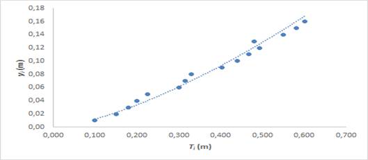
The behavior of the flow depth and the top width of the water on the furrow are presented in the Figure 1. These variables were adjusted appropriately to a model of simple potential type with a high coefficient of determination of 0.980; consequently, they can be used in a reliable way for estimating the flow depth in the furrow irrigation. This result is very important because it avoids the mensuration of the flow depth that is more annoying and inexact. The found model was the following:
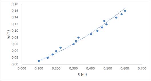
2071-0054-rcta-28-03-e04-gf1.jpg

FIGURE 1. 

Curves of the flow depth in function of top width.

Deduction of the Equation for Estimating Cross Sectional Area of the Flow in Furrows

The equation proposed in this investigation for estimating cross sectional area of flow in the furrow was sustained in the values of bottom width (b), top width (T), flow depth (y) and furrow side slope found experimentally. The sequence used for its deduction is presented next:

Substituting Equation (5) in (4) and clearing the parameter b, it is obtained:

Cross sectional area of flow in the furrow was assumed according to Cadavid (2009), as:

Substituting Equation (6) in (7), it is obtained:

Developing the previous equation is:

Cross sectional area of flow in function of the coefficient μ is obtained by means of the common factor:

Deduction of the Equation for Estimating Furrow Hydraulic Radius

Hydraulic radius of the furrow was determined as the quotient between cross sectional area of flow and wetted perimeter Gribbin (2016); this is:

Substituting Equation (10) and (13) in (14), it is obtained:

Simplifying, it is obtained:

The coefficient ξ is written in the following way:

Substituting Equation (17) in (16), the hydraulic radius is calculated in function of the coefficient ξ and flow depth of water in the furrow.

The inflow rate applied in the initial portion of the furrow was determined by means of continuity equation, which relates directly the cross sectional area of flow (A) and speed of the flow (v):

The estimation of water speed in the furrow irrigation was carried out from the Equation of Chezy and the speed coefficient by means of the Equation of Bazin (Roldán et al., 1999; Castanedo et al., 2013; Jiménez, 2015).The equations were the following:

Where C is the speed coefficient; S o the slope of the furrow (m m-1) and γ is the ruggedness coefficient of the furrow.

The substitution of the Equation (20) in the (19), an equation that facilitated the determination of the furrow inflow rate was obtained.

Analysis of Estimating the Flow Applied in the Furrow

The results of the methodology application, starting from an irrigation test in which a furrow inflow of 2.24 L·s-1 was applied and top width (T) was measured in the different stakes placed every 20 meters until the total furrow length of 100 m, are presented in Table 3. It is observed that the simulated furrow inflow rate is 2.24 L s-1 and it has a similar value to the applied real furrow inflow rate. This flow was obtained with a value of 3.64 for the Bazin ruggedness coefficient, which is in the range from 1.75 to 4.00, mentioned by Roldán et al. (1999).

TABLE 3. 

Value of hydraulic parameters measured and predicted in the furrows

X (m) T (m) y (m)μ A (m 2 )P m (m)ξR h (m)C v (m s -1 ) q (m 3 s -1 ) q (L s -1 )
00.450.11024.080.0280.5090.510.0565.300.0790.002242.24
200.420.09974.210.0240.4730.520.0525.120.0740.001801.80
400.360.07964.520.0180.4020.550.0444.720.0620.001101.10
600.300.06104.920.0120.3320.580.0354.280.0510.000600.60
800.280.05515.080.0100.3090.590.0334.120.0470.000480.48
1000.240.04405.450.0070.2630.620.0273.770.0390.000280.28

Table 3 shows that the flow diminishes when the advance front moves away from the initial portion of the furrow, what constitutes a normal behavior in this irrigation technique where the flow is variable and decreasing, as the distance increases. This is due to that the movement of the flow is not permanent (slowed) for the fact that the furrow inflow rate infiltrates in contact with the soil for the combined effect of the infiltration rate, ruggedness, furrow form and slope of the plot (Pacheco et al., 2007).

Comparison between real and simulated furrow inflow rate through the Average Percentage Error (APE) demonstrates that the proposed methodology is very exact for estimating furrow inflow rate that is applied in the furrows irrigation. That is evidenced in the fact that the APE obtained a value of 0.00% that indicates the absence of differences between both inflow rate.

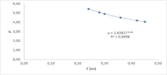
Functional relationship of the coefficients µ and ξ respect the top width is presented in Figures 2 and 3. The values of coefficients µ and ξ oscillated from 4.08 to 5.45 and of 0.51 to 0.62, respectively. In both cases, a simple potential model was achieved with high coefficients of determination of 0.9998 and 0.9996, respectively. That validates its sure application in the estimation of these coefficients for the calculation of cross sectional area of flow, the corresponding hydraulic radius.
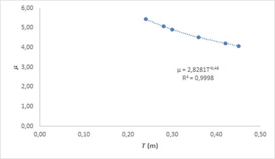
2071-0054-rcta-28-03-e04-gf2.jpg

FIGURE 2. 

Curve of coefficient μ respect top width.
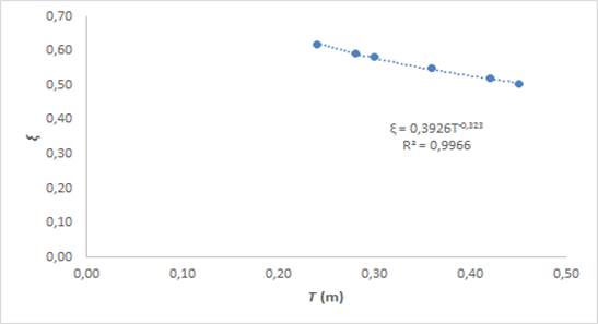
2071-0054-rcta-28-03-e04-gf3.jpg

FIGURE 3. 

Curve of coefficient ξ respect top width.

CONCLUSIONS

  • The geometric parameters of the furrow determined experimentally in sugar cane cultivation reached average values of 0.159 m; 0.590 m; 0.032 m and 1.756 for the maximum height of furrow, maximum top width, bottom width and side slope coeficient, respectively.

  • The simple potential model of type y=e·T f found in the investigation allows estimating, in a reliable way, the flow depth in the furrow from the direct mensuration of the top width.

  • The values of the coefficients µ and ξ oscillate from 4.08 to 5.45 and of 0.51 to 0.62, respectively. These are of great utility for the calculation of the cross sectional area of flow, only by estimating the side slope coeficient and flow depth in the furrow.

  • The proposed methodology demonstrated, through the Average Percentage Error, that the simulated flow is similar to the real furrow inflow rate and it confirms its high accuracy.


REFERENCES

BELLO, M.; PINO, M.: “Medición de presión y caudal”, Boletín INIA, Punta Arenas. Ministerio de Agricultura de Chile, 8: 21, 2000, ISSN: 0717-4829.

CADAVID, J.H.: Hidráulica de canales: fundamentos, Ed. Fondo editorial Universidad EAFIT, primera reimpresión ed., Medellín, Colombia, 2009, ISBN: 958-8281-28-8.

CARRIÓN, R.: Manual de captación: medición del agua de riego, Primera edición especial ed., Argentina, 31 p., 2015, ISBN: 978-987-33-8775-3.

CASTANEDO, V.; SAUCEDO, H.; FUENTES, C.: “Comparación entre un modelo hidrodinámico completo y un modelo hidrológico en riego por melgas”, Agrociencia, 47(3): 209-222, 2013, ISSN: 1405-3195.

DURÁN, P.J.; GARCÍA, P.M.: “Desarrollo de tecnologías apropiadas para riego por surcos en terrazas paralelas y tierras con pendiente”, Ingeniería del agua, 14(3): 187-198, 2007, ISSN: 1134-2196, e-ISSN: 1886-4996.

FACI, J.M.; PLAYÁN, E.: Principios básicos del riego por superficie, Ed. Ministerio de Agricultura Pesca y Alimentación, Secretaria General Técnica, Hojas divulgadoras, vol. 10-11, España, 32 p., 1996, ISBN: 84-491-0262-6.

GÉNOVA, L.J.; ANDREAU, R.; ETCHEVERS, P.: “Desempeño de tres métodos de riego por surcos: caudal único, dos caudales y caudal discontinuo en un cultivo de maíz”, Revista de la Facultad de Agronomía, La Plata, 113(2): 174-191, 2014, ISSN: 1669-9513.

GRIBBIN, J.E.: Introducción a la hidráulica e hidrología con aplicaciones para la administración del agua, Ed. Cengage Learning, México D. F., 543 p., 2016, ISBN: 978-607-526-003-7.

JIMÉNEZ, M.O.: “Fórmulas generales para los coeficientes de Chézy y de Manning”, Tecnología y Ciencias del Agua, 6(3): 33-38, 2015, ISSN: 2007-2422, e-ISSN: 0187-8336.

PACHECO, J.; ALONSO, N.; PUJOL, P.; CAMEJO, E.: Riego y Drenaje, Ed. Editorial Pueblo y Educación, segunda ed., La Habana, Cuba, 2007, ISBN: 978-959-07-0621-9.

PÉREZ, H.R.; JIMÉNEZ, E.E.; MONTERO, S.J.E.; GARCÍA, S.O.; GUZMÁN, V.J.: “Resultados de diferentes alternativas de manejo del riego superficial tecnificado en el cultivo de la papaya Maradol roja plantada con marco extradenso”, Revista Ingeniería Agrícola, 3(1): 8-16, 2013, ISSN: 2306-1545, E-ISSN: 2227-8761.

ROLDÁN, J.; PULIDO, I.; CAMACHO, E.; ALCAIDE, M.; LOSADA, A.: Problemas de hidráulica para riego, Ed. Servicios de Publicaciones de la Universidad de Córdoba, España, 284 p., 1999, ISBN: 84-7801-526-4.

SÁNCHEZ, A.; GARCÍA, N.P.; PLAYÁN, E.: “Modelo de simulación de riego por surcos inundados”, Ingeniería del agua , 9(3): 333-346, 2002, ISSN: 1134-2196, e-ISSN: 1886-4996.

SAUCEDO, H.; ZAVALA, M.; FUENTES, C.; CASTANEDO, V.: “Gasto óptimo en riego por melgas”, Tecnología y Ciencias del Agua , 4(3): 135-148, 2013, ISSN: 2007-2422, e-ISSN: 0187-8336.

VICENTE, S.S.M.; SAZ, S.M.A.; CUADRAT, J.M.: “Comparative analysis of interpolation methods in the middle Ebro Valley (Spain): application to annual precipitation and temperature”, Climate research, 24(2): 161-180, 2003, ISSN: 1616-1572, e-ISSN: 0936-577X.

ZÚÑIGA, A.; JORDÁN, C.: “Pronóstico de caudales medios mensuales empleando Sistemas Neurofuzzy”, Revista Tecnológica-ESPOL, 18(1): 17-23, 2005, ISSN: 1390-3659.


Oscar Brown Manrique, Profesor Titular, Universidad de Ciego de Ávila Máximo Gómez Báez, Facultad de Ciencias Técnicas, Centro de Estudios Hidrotécnicos, Ciego de Ávila, Cuba, e-mail: obrown@unica.cu

Daniubis Luis Pelier, Profesor, Universidad de Ciego de Ávila Máximo Gómez Báez, Facultad de Ciencias Técnicas, Departamento de Ingeniería Hidráulica, Ciego de Ávila, Cuba, e-mail: daniubis@unica.cu

Yurisbel Gallardo Ballat, Profesor Titular, Universidad de Ciego de Ávila Máximo Gómez Báez, Facultad de Ciencias Técnicas, Ciego de Ávila, Cuba, e-mail: yurisbel@unica.cu

The authors of this work declare no conflict of interest.

This article is under license Creative Commons Attribution-NonCommercial 4.0 International (CC BY-NC 4.0)

The mention of commercial equipment marks, instruments or specific materials obeys identification purposes, there is not any promotional commitment related to them, neither for the authors nor for the editor.


ARTÍCULO ORIGINAL


Metodología para la estimación del caudal aplicado en el surco a partir de las ecuaciones de Chezy y Bazin


RESUMEN

La investigación se desarrolló en la Unidad Básica de Producción Cooperativa Albio Hernández de la Empresa Azucarera Primero de Enero de la provincia de Ciego de Ávila. Los resultados demostraron que los parámetros geométricos del surco en el cultivo de la caña de azúcar alcanzaron valores promedios de 0,159 m; 0,590 m; 0,032 m y 1,756 para la altura máxima, el ancho superficial máximo, el ancho de la base y el coeficiente de talud respectivamente. El modelo potencial simple del tipo y=eT f permite la estimación de forma confiable del tirante de circulación del agua en el surco a partir de la mediación directa del ancho de la superficie libre del agua en el surco. Los valores de los coeficientes µ y ξ oscilan de 4,08 a 5,45 y de 0,51 a 0,62 respectivamente y resultan de gran utilidad para el cálculo del área de la sección transversal y el área hidráulica del surco. La metodología propuesta demostró a través del Error Porcentual Medio su elevada exactitud para la estimación del caudal aplicado en la entrada del surco.

Palabras clave: 

Coeficiente de rugosidad; hidráulica del riego por surcos; velocidad del agua.


INTRODUCCIÓN

El riego por superficie es el sistema de riego más empleado, ocupando la inmensa mayoría de las tierras de regadío a nivel mundial (Sánchez et al., 2002). En Cuba el riego superficial ocupa el 71% del área total irrigada y presenta un crítico estado tecnológico debido a la falta de inversiones para su mejoramiento (Pérez et al., 2013).

El riego superficial es intrínsecamente menos eficiente que la aspersión y el goteo, pues son inevitables las pérdidas por percolación profunda y por escurrimiento Génova et al. (2014); pero el diseño y manejo adecuado permite el riego eficiente y uniforme de la parcela (Faci y Playán, 1996; González y Playán, 1996).

En muchos países del mundo las investigaciones se llevan a cabo con el proposito de reemplazar el riego por surcos por metodos a presion; sin embargo, la situacion economico-financiera de los productores imposibilitan en muchas ocasiones realizar este tipo de cambio tecnologico, por lo que la alternativa posible es el riego superficial (Durán y García, 2007).

El conocimiento de la relacion entre el tipo de suelo, el agua y el cultivo permite la aplicación del agua en cantidades convenientes, según el sistema de riego a utilizar; es por eso, que la medicion del agua es esencial para el maximo aprovechamiento del recurso Carrión (2015); por otra parte, es necesario que el agricultor se familiarice con los términos asociados con la medición del caudal (Bello y Pino, 2000).

El diseño del riego consiste en determinar el caudal óptimo y el tiempo durante el cual se aplica dicho caudal en la cabecera del campo para lograr la mayor uniformidad de aplicación posible, para una longitud y un tipo de suelo en particular (Saucedo et al., 2013).

El objetivo del presente trabajo consiste en evaluar una metodología propuesta para la estimación del caudal aplicado en el riego por surcos a partir de las ecuaciones de Chezy y Bazin.

MÉTODOS

La investigación se desarrolló en una parcela sembrada de caña de azúcar de la variedad C-120 localizada en el bloque 609 de la Unidad Básica de Producción Cooperativa (UBPC) Albio Hernández de la Empresa Azucarera Primero de Enero, de la provincia Ciego de Ávila. El sistema de riego empleado es del tipo riego por surcos mediante tuberías multicompuertas formado por una tubería soterrada de PVC con diámetro de 315 mm que sale directamente de la estación de bombeo con una longitud máxima de 500 m en la cual se colocan los hidrantes que suministran el agua a las tuberías de riego de PVC con diámetro de 280 mm. Esta tiene compuertas regulables cada 1,50 m para la descarga del caudal en el surco.

La altura máxima del surco (y max ), el ancho superficial máximo (T max ) y el ancho de la base (b) se midieron en condiciones experimentales en nueve surcos seleccionados al azar dentro del área de estudio; posteriormente el coeficiente de talud del surco se obtuvo mediante la ecuación siguiente:

El caudal suministrado al surco se midió a la salida de las compuertas con la utilización del método volumétrico; luego se registraron los tiempos en que el frente de avance del flujo de agua alcanzó las estacas colocadas a equidistancias de 20 metros sobre una la longitud total del surco de 100 m y pendiente promedio de 4,0‰. Se empleó un cronómetro digital con precisión de un segundo. En estos puntos se obtuvo además el valor del ancho superficial del agua (T i ) y el tirante (y i ) lo que permitió encontrar un modelo de ajuste para la estimación del tirante en función del ancho superficial del agua.

La validación de los modelos estadísticos se realizó mediante el Coeficiente de Determinación (R 2 ) según Vicente et al. (2003) y el Error Porcentual Medio Zúñiga y Jordán (2005), con series de datos diferentes utilizadas convenientemente para la generación del modelo y el pronóstico. La ecuación utilizada fue la siguiente:

Donde EPM es el Error Porcentual Medio (%); n el número de datos de la serie; y obs la variable observada; y sim la variable simulada.

La metodología propuesta en esta investigación se compone de seis procedimientos fundamentales: (1) determinación práctica del coeficiente de talud de los surcos de riego; (2) determinación del modelo que relaciona el tirante con el ancho superficial del agua en el surco; (3) obtención de los coeficientes μ y ξ para la estimación del área hidráulica, el perímetro mojado y el radio hidráulico del surco; (4) estimación de la velocidad del agua en el surco de riego según la ecuación de Chezy y el coeficiente de velocidad por la ecuación de Bazin; (5) cálculo del caudal de entrada al surco mediante la ecuación de continuidad y (6) validación de la metodología propuesta a través de la comparación entre los caudales reales aplicados y los simulados.

RESULTADOS Y DISCUSIÓN

Análisis del coeficiente de talud en los surcos de riego

En la Tabla 1 se exponen los valores de los parámetros geométricos del surco obtenidos directamente en los diferentes puntos de muestreos establecidos en el área experimental. En la Tabla 2 se muestra los principales estadígrafos correspondientes al análisis descriptivo, donde se destacan los valores medios de la altura máxima, del ancho superficial máximo, del ancho de la base y del coeficiente de talud con 0,159 m; 0,590 m; 0,032 m y 1,756 respectivamente, por lo que deben tomarse como parámetros de diseño definitivo para las condiciones específicas de este sistema productivo.

TABLA 1. 

Parámetros medidos en el surco para la determinación del coeficiente del talud.

Noy max (m)T max (m) b (m)
10,1600,6000,028
20,1650,6000,033
30,1600,5850,035
40,1500,5630,024
50,1400,5700,042
60,1700,6140,030
70,1540,5800,030
80,1660,6100,029
90,1700,5870,037

TABLA 2. 

Estadística descriptiva de los parámetros geométricos del surco.

Estadígrafoymax (m)Tmax (m)b (m)m
Media0,1590,5900,0321,756
Error típico0,0030,0060,0020,025
Mediana0,1600,5870,0301,750
Moda0,1600,6000,0301,720
Desviación estándar0,0100,0170,0050,075
Varianza de la muestra0,000100,000300,000030,00558
Curtosis0,304-1,0790,2611,248
Coeficiente de asimetría-0,902-0,1270,550-0,010
Rango0,0300,0510,0180,270
Mínimo0,1400,5630,0241,620
Máximo0,1700,6140,0421,890

Obtención de modelo que relaciona tirante con el ancho superficial del agua en el surco

En la Figura 1 se presenta el comportamiento del tirante de circulación del agua y el ancho de la superficie libre del agua sobre el surco. Estas variables se ajustaron adecuadamente a un modelo de tipo potencial simple con un coeficiente de determinación elevado de 0,980; por lo que puede ser utilizado de forma confiable para la estimación del tirante de circulación del agua en el surco en un sistema de riego por gravedad. Este resultado es muy importante; porque se evita la medición del tirante de circulación que es más engorroso e inexacto. El modelo encontrado fue el siguiente:

2071-0054-rcta-28-03-e04-gf4.jpg

FIGURA 1. 

Curva del tirante en función del ancho superficial del agua en el surco.

Deducción de la ecuación para la estimación del área hidráulica del surco

La ecuación para la estimación del área hidráulica del surco propuesta en esta investigación se sustentó en los valores de ancho de la base del surco (b), ancho superficial de la superficie libre del agua (T), tirante de circulación del agua (y) y coeficiente de talud del surco (m) encontrado experimentalmente. La secuencia utilizada para su deducción se expone seguidamente:

Sustituyendo la ecuación (5) en la (4) y despejando el parámetro b, se obtiene:

El área hidráulica del surco (A) se asumió según (Cadavid, 2009), como:

Sustituyendo la ecuación (6) en la (7) se obtiene:

Desarrollando la ecuación anterior queda:

Sacando factor común se obtiene la ecuación que permite calcular el área hidráulica del surco en función del coeficiente μ:

Deducción de la ecuación para la estimación del radio hidráulico del surco

El radio hidráulico del surco (R h ) se determinó como el cociente entre el área hidráulica y el perímetro mojado Gribbin (2016); esto es:

Con la sustitución de las ecuaciones (10) y (13) en la (14) se obtiene:

Simplificando queda:

Se supone un coeficiente ξ que se escribe de la siguiente forma:

La sustitución de la ecuación (17) en la (16) permite calcular el radio hidráulico en función del coeficiente ξ y el tirante de circulación del agua en el surco.

El caudal aplicado en el extremo inicial del surco (q) se determinó mediante la ecuación de continuidad, la cual relaciona de forma directa el área hidráulica de la sección transversal del surco (A) y la velocidad del flujo (v):

La estimación de la velocidad del agua en el surco de riego se realizó a partir de la ecuación de Chezy y el coeficiente de velocidad para la ecuación de Bazin (Roldán et al., 1999; Castanedo et al., 2013; Jiménez, 2015). Las ecuaciones fueron las siguientes:

Donde C es el coeficiente de velocidad; S o la pendiente del surco (m m-1); γ el coeficiente de rugosidad del surco.

Con la sustitución de la ecuación (20) en la (19) se obtuvo la ecuación que posibilitó la determinación del caudal aplicado en el surco.

Análisis de la estimación del caudal aplicado en el surco

En la Tabla 3 se exponen los resultados de la aplicación de la metodología a partir de una prueba de riego en la que aplicó un caudal de entrada de 2,24 L s-1 y se midió el ancho de la superficie libre del agua (T) en las diferentes estacas colocadas cada 20 metros hasta la longitud total de 100 m. Se observa que el caudal simulado a la entrada del surco es de 2,24 L s-1 y presenta un valor igual al caudal real aplicado. Este caudal se obtuvo con un valor de 3,64 para el coeficiente de rugosidad de Bazin, el cual se encuentra en el rango de 1,75 a 4,00 mencionado por Roldán et al. (1999).

TABLA 3. 

Valores de los parámetros hidráulicos del surco medidos y estimados.

X (m) T (m) y (m)μ A (m 2 )P m (m)ξR h (m)C v (m s -1 ) q (m 3 s -1 ) q (L s -1 )
00,450,11024,080,0280,5090,510,0565,300,0790,002242,24
200,420,09974,210,0240,4730,520,0525,120,0740,001801,80
400,360,07964,520,0180,4020,550,0444,720,0620,001101,10
600,300,06104,920,0120,3320,580,0354,280,0510,000600,60
800,280,05515,080,0100,3090,590,0334,120,0470,000480,48
1000,240,04405,450,0070,2630,620,0273,770,0390,000280,28

En la propia Tabla 3 se observa que el caudal disminuye en la medida que el frente de avance se aleja del extremo inicial del surco, lo que constituye un comportamiento normal en esta técnica de riego donde el caudal es variable y decreciente, a medida que aumenta la distancia. Esto se debe a que el movimiento del flujo es no permanente (retardado) por el hecho de que el caudal suministrado al surco se infiltra en contacto con el suelo por el efecto combinado de la tasa de infiltración, la rugosidad, la forma del surco y la pendiente del terreno (Pacheco et al., 2007).

La comparación entre el caudal real aplicado y el simulado a través del Error Porcentual Medio (EPM) demuestra que la metodología propuesta es muy exacta para la estimación del caudal que se aplica en el riego por surco, lo cual se evidencia en el hecho de que el EPM obtuvo un valor de 0,00 %, que indica la ausencia de diferencias entre ambos caudales.

En las Figuras 2 y 3 se presenta la relación funcional de los coeficientes µ y ξ con respecto al ancho de la superficie libre del agua en el surco. Los valores de los coeficientes µ y ξ oscilaron de 4,08 a 5,45 y de 0,51 a 0,62 respectivamente. En ambos casos se logró un modelo potencial simple con elevados coeficientes de determinación de 0,9998 y 0,9996 respectivamente, lo que avala su aplicación segura en la estimación de estos coeficientes para el cálculo del área de la sección transversal del surco, el radio hidráulico correspondiente.

2071-0054-rcta-28-03-e04-gf5.jpg

FIGURA 2. 

Curva del coeficiente μ respecto al ancho superficial del agua en el surco.

2071-0054-rcta-28-03-e04-gf6.jpg

FIGURA 3. 

Curva del coeficiente ξ respecto al ancho superficial del agua en el surco.

CONLUSIONES

  • Los parámetros geométricos del surco determinados experimentalmente en el cultivo de la caña de azúcar alcanzaron valores promedios de 0,159 m; 0,590 m; 0,032 m y 1,756 para la altura máxima, el ancho superficial máximo, el ancho de la base y el coeficiente de talud respectivamente.

  • El modelo potencial simple del tipo y=eT f encontrado en la investigación permite la estimación de forma confiable del tirante de circulación del agua en el surco a partir de la medición directa del ancho de la superficie libre del agua en el surco.

  • Los valores de los coeficientes µ y ξ oscilan de 4,08 a 5,45 y de 0,51 a 0,62 respectivamente. Estos resultan de gran utilidad para el cálculo del área de la sección transversal y el área hidráulica del surco con solo estimar el coeficiente de talud y el tirante de circulación del agua en el surco.

  • La metodología propuesta demostró a través del Error Porcentual Medio que el caudal simulado es igual al caudal real aplicado en la entrada del surco; por lo que se confirma su elevada exactitud.