INTRODUCTION
Historically, the study of the dynamics of agrarian processes has been accompanied by algebraic expressions, but because they are very complex systems by nature, at first they could not be solved by the traditional methods of Mathematical Analysis. In practice, these phenomena have evolved, and in many cases, they were represented through Mathematical Statistical Models, which allow describing processes, perform detailed quantitative analyses, predict the behavior of objects in different conditions, and develop techniques that allow establishing work strategies to achieve optimal solutions and productions.
Statistical-Mathematical Modeling and its applications in Agrarian Sciences, have been present for more than 40 years at the Agrarian University of Havana and researching in collaboration with Institute of Animal Science (ICA), National Center for Agricultural Health (CENSA) and National Institute of Agricultural Sciences (INCA). They have worked biometry and modeling of agrarian and biological processes. This is corroborated in the works of Menchaca (1978, 1990), in studies of lactation curves in dairy cows, in which he used a multiplicative model with effects of these curves, in parallel. Guerra (1980), used the Response Surface Methodology (MSR) in crops of sugarcane, citrus fruits, pastures and fodder, to explore the optimal conditions of fertilization.
Menchaca (1990), used models called staged or by steps, to describe animal growth curves, and in the work of Del Pozo and Herrera (1995), the use of multiplicative models with control of growth curves and environmental effects in star grass (Cynodon nlemfumsis) growth studies is reported.
Fernández (1996, 2004), conducted a study associated with Mathematical Models that describe the dynamics of biological processes in agricultural sciences, with emphasis on nonlinear regressions and the use of iterative methods for the estimation of parameters and not by the linearization of the model as it had traditionally been worked. The development of computer science and statistical softwares facilitated the work of non-linear regressions in this way. More recently, Fernández et al. (2018), exposed the evolution in nonlinear regressions and the proposal of initial parameters from mathematical-biological interpretations of them; she also reported examples ranging from animal and plant growth models, allometric growth and lactation curves, among other processes.
Likewise, models associated with genetic evaluations and improvements in cattle (with the use of the BLUP (Best Linear Unbiased Predictor) and the use of weighing in the control day), as well as pasture growth models (King Grass) have been approached for the determination of the optimum cutting moment (Rodríguez, 2015). Other researches in the area of Agricultural Sciences have been reported by Fernández (1996a, 1996b, 2004), Del Valle (2000), Del Valle and Guerra (2012) and Vázquez et al. (2014), among others.
In Agricultural Technical Sciences, Mathematical Modeling has been applied to the prediction of quality properties of Rangel fruits (2015), in which linear and non-linear models are involved in the characterization of these processes. The theoretical basis of the most used models are addressed in this work. For the interest of this topic and its impact on research, the present review was developed to establish criteria and assessments in the analysis and application of models that describe agrarian processes, on mathematical - statistical bases.
METHODS
Theoretical fundament
Linear models
The best-known case of Mathematical Models is the linear model, which is expressed in a general way as:
Yi
- Dependent variable or response.
ßj
- Parameters of the model (j = 0,1,2 ... p)
x ji
- i-th value of the independent variable (j = 1,2,3, ..., p).
ei
- independent random error, with normal distribution with zero mean and variance σ2
The concept of linearity and non-linearity is referred to the parameters. In this case, (x) is considered as a constant, and the dependence of (Y) with the parameters is a combination of addition and subtraction. Menchaca (1990), when referring to linear models, points out that they present limitations from the practical and biological points of view, but they are extremely useful if the objective corresponds more to the field of estimation than to biological interpretation. In addition, these are very used by the simple mathematical method they utilize to estimate their parameters (method of ordinary least squares), which is accurate, and the solution is unique.
The general model can be taken to specific forms. Some of them are the first order polynomial, second order polynomial, and the like. Among the linear models that have shown good level of adjustment in applications within agricultural technical sciences, the cubic and polynomial logarithmic polynomial can be mentioned, whose fundamental characteristics and functional form are shown in Table 1.
TABLE 1.
Summary of useful aspects of linear models
| Model | Functional Form | First Derivative | Inflection Point |
|---|---|---|---|
| 1 | |||
| 2 |
1- Cubic polynomial 2-polynomial logarithmic
Yi- Dependent variable.
ßj - Parameters of the model (j = 0,1,2, ..., p)
xi - i-th value of the independent variable.
ei - independent random error, with normal distribution, with zero mean and variance σ2
Non-Linear Models
Although linear models are suitable for many situations, some variables are not connected to each other by a simple relationship, such as the algebraic representation of the growth dynamics of individuals in animal species or the kinetics of postharvest weight loss. This has led to the search and construction of mathematical models, which have turned out to be non-linear in many cases.
The disadvantage of these models is that for the calculation of their parameters, iterative methods are used, and this leads to very complex calculations and can even fall into errors when estimating the parameters. Many authors use transformations to linearize the model and apply the minimum method square, but in practice, this procedure is not advisable. At present, there are specific programs for non-linear adjustment, which allow overcoming this disadvantage.
Within the non-linear models frequently used are those that are asymptotic without inflection points (Models of Brody, Modified Exponential) and those that are asymptotic with inflection points (Models of Gompertz, Von-Bertalanffy, and Logistic, among others). Table 2 shows the algebraic expressions of some of these models, as well as indicators associated with the calculation of speed and / or the rate of profit (first derivative), point of inflection.
TABLE 2.
Functional form and aspects related to non-linear models
f (t): Dependent random variable, t: Independent variable, controlled or predefined, A, b, k: parameters to be estimated.
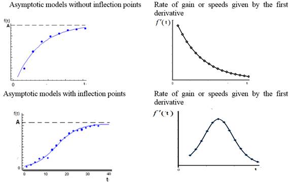
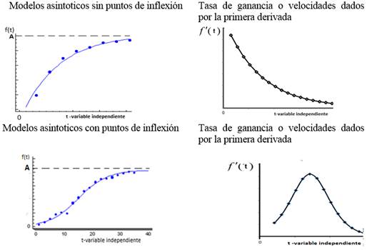
In the Brody model, the function is concave and grows until its value stabilizes as the value of t increases; however, the velocities or rates (f l (x)) decrease as the value of t increases. (Figure 1)
The shape of the rest of the models is sigmoid. The difference between them is the location of the inflection point. The speeds or rates in these models is flared; this increases until it reaches its maximum value, and then decreases to zero. (Figure 1)

FIGURE 1.
Representation of non-linear models and their corresponding rates or speeds.
Application of These Models in Studies of Post-Harvest Curves of Pineapple (variety Cayena Lisa)
The study was carried out in areas of the company of several crops located within the Havana-Matanzas Plain, with a range of average annual temperature between 25 and 32 ºC and high humidity. Weight Loss (PP) was performed through the weighing of fruits with the use of the electronic balance, during the first nine days after harvesting. Average values (g) were calculated on the days observed. The Logistics and Von Vertalanffy models (described above) were tested. For the goodness of fit and discrimination between models, the coefficient of determination, sum of the square of the error, significance of the model and the parameters, distribution of the residuals and Durbin Watson's hypothesis test were taken into account. The loss process is described from the best model. The speed with which the weight loss occurs at each instant of the period analyzed is estimated from the derivative of the function, and the search of the moment where the maximum speed of weight loss occurred was calculated by the inflection point.
RESULTS OBTAINED
The average values of weight loss (g) and the corresponding days allowed us to estimate the parameters of the adjusted curves (Table 3), which showed good adjustment with coefficient of determination above 97%. This indicates that both models are an alternative for the description of the process and for the prediction within the range of values studied.
The discrimination between the models allowed selecting the Logistic Model as the best one, which explains 99.27% of the total variability. All its parameters are significant and it achieved lower standard error of estimation, absolute mean of the error and sum of squared of the error than the model of Von - Bertalaffy (Table 3).
TABLE 3.
Result of the adjustment of the models
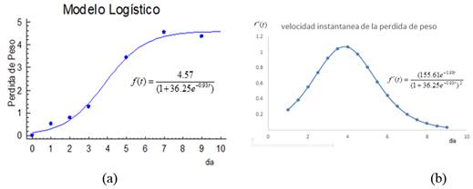
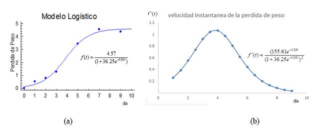
The Logistic model selected (Figure 2a) shows the increase in weight loss as the post-harvest day’s increase, with abrupt behavior during the first days and a tendency to stabilize this value from the seventh day. This trend described by the model is considered adequate and is associated, among other aspects, with the irreversible physiological changes that occur in the fruit.
Another indicator of interest is associated to the behavior of the speed with which this weight loss occurs (Figure 2b), which is in flared form. This increases until reaching its maximum value, approximately on the fourth day, and then decreases to zero.

FIGURE 2.
Model of best fit for weight loss (2a) and speed with which it occurs (2b).
Table 4 shows the inflection point (3.8, 2.24) which is where the maximum speed of weight loss is reached. It was of 1.07 g. It also shows the values reached around this point.
TABLE 4.
Behavior of the weight loss and the speed with which the weight loss occurs around the inflection point
| Day | 3.5 | 3.6 | 3.7 | 3.8 | 3.9 | 4 | 4.1 | 4.2 |
|---|---|---|---|---|---|---|---|---|
| Weight Lossing (g) | 1.927 | 2.032 | 2.138 | 2.245 | 2.352 | 2.459 | 2.565 | 2.669 |
| Speed of PP (g) | 1.046 | 1.060 | 1.068 | 1.073 | 1.072 | 1.067 | 1.058 | 1.044 |
These indicators associated with the loss of weight, are of special interest to save resources, time and efforts, which allows tracing postharvest handling strategies and guarantee the quality of the product.
Currently, there are valuable results regarding the use of these and other types of models that have been used to predict the production of green and dry grass biomass (Maralfalfa). They have been studied with several doses of nitrogen fertilizer; or in the description and characterization of the physical and chemical properties of the pineapple (variety Cayenne Lisa) stored at room temperature. Moreover, they have been used in the modeling and simulation of the star grass (C. nlemfuensis) performance under different management conditions and climatic scenarios (Fernández et al., 2011; Rangel, 2015; López, 2016 and others).
CONCLUSIONS
To deal in detail with the analysis of agrarian processes, knowledge of a group of models is required with the application of Differential Calculus and Mathematical Statistics, among other aspects.
The graph of different models, as well as their absolute rates, help to clarify the analysis of the dynamics of different agrarian phenomena.
Mathematical modeling allows deepening the laws that govern each of the phenomena, facilitates the study of the process and creates a methodological basis for the processing of information
It is concluded that the development of Statistical-Mathematical Modeling allows responding to current problems of research in the agricultural sector and to the teaching and scientific-research challenges of the new University.


