Study area

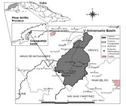
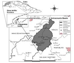
The study focuses on the “V Aniversario” subwatershed, which is one of the natural hydrographic closures of Cuyaguateje River basin, located in Pinar del Río Province. This subwatershed extends over part of Viñales and Minas de Matahambre Municipalities, with an extension of 157 km² and is located at 22º24’6”N - 22º35’40”N and 83º47’55”O - 83º56’9”O. Figure 1 shows the geography of the study area. Its latitudinal position favors the development of a volume of runoff, which is higher than other karstic regions in the country. In particular, given its geomorphological drainage (soil) and coverage characteristics, it presents a rapid response in form of floods (Consejo Territorial de Cuencas Hidrográficas (CTCH) de Pinar del Río, 2000).

Discharge Series

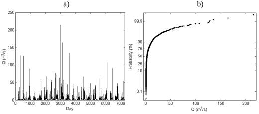
Discharge series was used to calibrate and validate the physically-based model. These variables are monitored at the subwatershed’s outlet (“V Aniversario” hydrometric station) by the traditional methods, using a current meter and the water level is also monitored continuously with a limnimeter. The data available for this study were daily mean discharge rates in the period from 1971 to 1990 (Alonso, 2016). It is interesting to notice that, in this period, the hydrometric station of “V Aniversario” subwatershed has recorded an annual runoff average of 3,72 m³/s, an observed maximum of 453 m³/s and the monthly mean varies between 0,7 and 8,9 m³/s (Consejo Territorial de Cuencas Hidrográficas (CTCH) de Pinar del Río, 2000). In this study, the daily mean values were approximately converted into annual and monthly mean values. In the case of the annual mean values, the conversion was made finding the mean of all the daily mean values in each year. Figure 2a shows the average daily runoff, as well as the empirical cumulative density function (Figure 2b).

Linear Stochastic Models

Linear stochastic modeling of runoff in rivers results in a hydrological response that is predicted from the previous steps. White Noise and ARMA models (Metcalfe y Cowpertwait, 2009): autoregressive (AR(p)), moving average (MA(q)) and its variants allow obtaining additional information about time series, such as seasonality. Due to the importance of these models to arrive to the results in this article, they will be briefly discussed below.

White Noise (WN). A residual error is the difference between the observed value and the model predicted value at time t. If we suppose the model is defined for the variable y _t and ŷ _t is the value predicted by the model, the residual error x _t is

As the residual errors occur in time, they form a time series: x ₁ ,x ₂ ,…,x _n .

Autoregressive Model AR(p). The series {x _t } is an autoregressive process of order p, abbreviated to AR(p), if:

Eq. 2 can be expressed as a polynomial of order p in terms of the backward shift operator (B):

The current value of the series xt is a linear combination of the most recent past p values of itself plus an “innovation” term wt that incorporates everything new in the series at time t, that is not explained by the past values (Cryer y Chan, 2010).

Moving Average Model MA(q). A moving average (MA) process of order q is a linear combination of the current White Noise term and the most recent past q terms of White Noise. This is defined by

Eq. 4 can be rewritten in terms of the backward shift operator B and ϕq polynomial of order q as:

Because MA processes consist of a finite sum of stationary White Noise terms, they are stationary and hence have a time-invariant mean and autocovariance.

Autoregressive Moving Angle Expression. A time series {xt} follows an autoregressive moving average (ARMA) process of order (p, q), denoted ARMA(p, q), when

Eq. 6 may be represented in terms of the backward shift operator B and rearranged in the more concise polynomial form:

Statistical Analysis Used

For arriving to favorable results, it is necessary to make choices based on statistical criteria and tests. Then, Akaike´s Information Criterion (AIC) of Shumway and Stoffer (2011)and the Mann-Kendall trend test according to Wilks (2011), are described. They are fundamental in this article.

Akaike's Information Criterion (AIC). This criterion is given by the following definition:

σ̂ _k ² is given by:

SSE _k denotes the residual sum of squares under the model with k regression coefficients.

The value of k that yields the minimum AIC species is the best model. The idea is roughly minimizing σ̂ _k ², which would be a reasonable objective, except that it decreases monotonically as k increases. Therefore, it is necessary to penalize the error variance by a term proportional to the number of parameters. The choice for the penalty term, in this case, is given by Eq. 8.

Mann-Kendall Trend Test. This test is a popular nonparametric alternative for testing for the presence of a trend, or for a non-stationary central tendency of a time series. In the context of examining the possibility of trend underlying a time series x _i , where i is the time index and it takes values i=1,…,n, the trend is, by definition, monotonically increasing, which simplifies the calculations.

The test statistic for the Mann-Kendall trend is

where

For moderate (n about 10) or larger series lengths, the sampling distribution of the test statistic in Eq. 10 is approximately Gaussian, and if the null hypothesis (no trend) is true, this Gaussian null distribution will have zero mean. The variance of this distribution depends on whether all the x’s are distinct, or if some are repeated values.

Annual Discharge Series

The representation of the annual runoff series of the "V Anniversary" subwatershed is shown in Figure 3a. In this series also appears the non-parametric Mann-Kendall test results for significance of the slope (pval). In Figure 3b, the normality graph is observed.

In the plotted time series, it can be seen that there is not a significant trend. In the Mann-Kendall test, the null hypothesis (H₀) corresponds to no trend, which is corroborated by the result of the pval (much higher than 0.05). In addition, the distribution of the series, assumed with random variables, is very close to normal, with small deviations in the tail. In general, the series can be considered as stationary.

Table 1 summarizes the basic descriptive statistics for the analyzed series at annual scale. According to the skewness (1.41) that is greater than zero, it is determined that the series is right skewed, typical pattern of the hydrological series.

In Figure 4, the autocorrelation (ACF) and partial autocorrelation (PACF) functions of the series are shown. It can be concluded from these graphs that this series behaves like a pure White Noise, because there is not a significant temporal correlation between years, that is, none of the orders (lag) has a correlation value that exceeds the dashed lines (significance test), with values of approximately ±0,4. Only the zero order, in Figure 4a, has a correlation value of one, but this order means null phase shift, so it is concluded that there is not temporal memory in the system that can be exploited. Therefore, the process, at this scale, is explained by the random component.

The result shown by the previous graphs (Figure 4), can be corroborated by Figure 5, where the Akaike's Information Criterion (AIC) is represented for an AR(p) y MA(q), respectively. In the case of the AR(p) (Figure 5a), the only significant value is obtained for the zero order, so it is meaningless to use this modeling structure. However, for the MA(q) in order three (Figure 5b), it seems to be an indication of a possible explanation of the variability of the series. This variability can be associated to the interannual variability of the precipitations and, therefore, of the runoff as a response of them. Specifically, the effects of ENOS (El Niño South Oscillation), an atmospheric phenomenon that influences the climatic conditions of the Caribbean, provoke cycles between three and four years, as average. The results in the AIC maybe reflect this context. However, there are not enough elements to conclude that, the amount of values analyzed seems to be still insufficient for detecting a correlation in this phenomenon that is cyclical, but erratic. On the other hand, Akaike penalizes the models by the number of parameters, which in this case is three, and, as it can be observed in Figure 5b, the MA(3) model does not have better AIC in comparison with the MA(0) or White Noise. In addition, the results of this criterion for the order three are corroborated by the ACF and PACF graphics, where it is demonstrated, for this order, that there is not practically correlation. Therefore, it is considered that the best model that represents the behavior of this series is the White Noise, as it had already been expressed previously. However, this is not in correspondence with what Aviles et al. (2016) obtained, where several models were tested at annual scale and according to the AIC, the best model that was adjusted to their data series was the ARMA (1,1). On the other hand, according to Díaz and Guevara (2016), the appropriate model for describing the annual average flows in watersheds of Santa river, Peru is the AR (1).

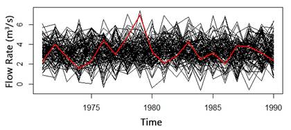
Table 2 shows the observed runoff statistic and White Noise generations. In this case, the model reproduces the statistical measurements very well. Figure 6, known as “spaghetti” graph, represents the 100 series that were generated by the White Noise, where the observed data series appears in red. Therefore, the synthetic and observed realizations, which emerge from the same process, can be visually compared.

Monthly Discharge Series

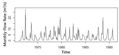
Due to the limited temporal memory that was found in the annual runoff series, it was decided to explore the monthly scale. Figure 7 shows monthly runoff series of “V Aniversario” watershed. In addition, observed values and the decomposed elements of the time series: trend, seasonality and randomness, are represented in Figure 8a. The main component to take into account in this series is seasonality. From Figure 8b, it is evident that data are distributed approximately normal, only with small deviations in the tails, as it happened at annual scale.

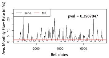
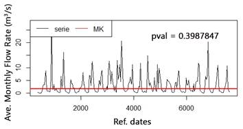
Another similarity between this series and the series at annual scale, is that both have a p value higher than 0.05, then it can be proved that there is not trend in the series, in the period studied, according to the Mann-Kendall Trend Test (Figure 9).

Table 3 summarizes the fundamental descriptive statistic for analyzing the time series at monthly scale, being this series right skewed, in accordance with the annual. On the other hand, Figure 10 shows the autocorrelation (ACF) and partial autocorrelation (PACF) functions. As it is expected, memory or persistence is much higher in shorter periods in runoff observations, which is in correspondence with the study carried out by Valipour et al. (2013), at this same scale. Therefore, the significant linear correlation, with different steps back in time, is very superior in the monthly measurements compared with the annual ones, despite the influence of the sample size on the confidence limits. The seasonality of the monthly series can be easily recognized in these graphs. The linear correlation coefficient, either positive or negative, alternates every 6 months.

From the previous graphs, the seasonality of the monthly runoff series is corroborated. That is why an appropriate model for the series would be a seasonal autoregressive integrated moving average (SARIMA). SARIMA has six parameters: p, d, q, P, D y Q, then it is more complex than ARMA models.

Área de Estudio

El estudio se centra en la subcuenca “V Aniversario”, que es uno de los cierres hidrográficos naturales de la cuenca del Río Cuyaguateje, ubicada en la provincia de Pinar del Río. Esta subcuenca abarca parte de los municipios de Viñales y Minas de Matahambre, con una extensión de 157 km² y se localiza en los 22º24’6”N - 22º35’40”N y 83º47’55”O - 83º56’9”O. La Figura 1 muestra la geografía del área de estudio. Su posición latitudinal favorece el desarrollo de un volumen de escurrimiento superior a otras corrientes en zonas cársicas del país. En particular, dadas sus características geomorfológicas, de drenaje (suelo) y cobertura, presenta pronta respuesta en forma de avenidas (Consejo Territorial de Cuencas Hidrográficas (CTCH) de Pinar del Río, 2000).

Series de escurrimiento

La serie de escurrimiento fue usada para calibrar y validar el modelo de base física. Estas variables son monitoreadas en la desembocadura de la subcuenca (estación hidrométrica V Aniversario) por los métodos tradicionales, usando molinete y la medición constante del nivel con un limnímetro. El dato disponible para este estudio es el escurrimiento medio diario, medido durante el período de 1971 a 1990 (Alonso, 2016). Es de interés destacar que, en este período, la estación hidrométrica de la subcuenca V Aniversario ha registrado un escurrimiento medio anual de 3,72 m³/s y un máximo observado de 453 m³/s, la media mensual oscila entre 0,7 y 8,9 m³/s (Consejo Territorial de Cuencas Hidrográficas (CTCH) de Pinar del Río, 2000). En este estudio, los valores medios diarios fueron convertidos, aproximadamente, en valores medios anuales y mensuales. En el caso de los valores medios anuales, la conversión se realizó hallando la media de todos los valores medios diarios en cada uno de los años. En la Figura 2a se refleja el escurrimiento medio diario, así como la función empírica de densidad acumulada (Figura 2b).

Modelos lineales estocásticos

La modelación lineal estocástica del escurrimiento en ríos da como resultado una respuesta hidrológica que se predice a partir de los pasos anteriores. Los modelos de Ruido Blanco y de la familia ARMA (Metcalfe y Cowpertwait, 2009): autorregresivos (AR(p), por sus siglas en inglés), de media móvil (MA(q), por sus siglas en inglés) y sus variantes, permiten obtener información adicional acerca de las series de tiempo, como su comportamiento estacional. Debido a la importancia que tienen estos modelos para arribar a los resultados en este artículo, se abordarán brevemente a continuación.

Ruido blanco (WN). Un error residual es la diferencia entre el valor observado y el valor predicho por el modelo en un tiempo t. Si se supone que el modelo es definido por la variable y _t y ŷ _t es el valor predicho por el modelo, el error residual x _t es:

Como los errores residuales ocurren en el tiempo, ellos forman una serie temporal: x ₁ ,x ₂ ,…,x _n .

Modelo autorregresivo AR(p). La serie {x _t } es un modelo autorregresivo de orden p, abreviado como AR(p), si:

La Ec. 2 puede ser expresada como un polinomio de orden p en términos del operador de retroceso hacia atrás (B):

El valor de la serie xt es una combinación linear de los p valores pasados más recientes de sí misma, más un término de “innovación” wt que incorpora todo lo nuevo en la serie en un tiempo t, que no es explicado por los valores pasados (Cryer y Chan, 2010).

Modelo de media móvil MA(q). Un modelo de media variable (MA) de orden q es una combinación lineal del término actual de Ruido Blanco y de los q términos pasados más recientes de Ruido Blanco. Este es definido como:

La Ec. 4 puede ser nuevamente escrita en términos del operador de retroceso hacia atrás B y del polinomio ϕq de orden q como:

Debido a que los procesos MA consisten en una suma finita de términos estacionarios de Ruido Blanco, son entonces estacionarios y, por lo tanto, tienen una media y autocovarianza invariantes en el tiempo.

Modelo autorregresivo de media móvil ARMA(p,q). Un modelo muy útil es obtenido cuando los términos del AR y MA son juntados en una sola expresión. Una serie de tiempo {xt} sigue un modelo autorregresivo de media variable (ARMA) de oden (p, q), denotado como ARMA(p, q), cuando:

La Ec. 6 puede ser representada en términos del operador de retroceso hacia atrás B y puede ser reajustada en la forma de un polinomio más conciso:

Análisis estadístico usado

Para arribar a resultados favorables, es necesario realizar elecciones basadas en criterios y test estadísticos. A continuación, se describen el Criterio de Información Akaike (AIC, por sus siglas en inglés) de Shumway y Stoffer (2011) y el test de tendencia de Mann-Kendall, según Wilks (2011), los cuales son fundamentales en este artículo.

Criterio de información Akaike (AIC). El criterio está dado por la siguiente definición:

σ̂ _k ²está dado por:

SSE _k denota la suma residual de cuadrados en el modelo con k coeficientes de regresión.

El valor de k que arroje el AIC mínimo, es el mejor modelo. La idea es minimizar σ̂ _k ², lo cual sería un objetivo razonable si este no decreciera monótonamente a medida que k se incrementa. Entonces, se necesita penalizar la varianza del error por un término proporcional al número de parámetros. La elección del término de penalización, en este caso, está dada por la Ec. 8.

Test de tendencia de Mann-Kendall. Este test es una alternativa no paramétrica popular para probar la presencia de una tendencia, o que la tendencia central sea no estacionaria, de una serie temporal. En el contexto de examinar la posibilidad de tendencia que corresponde a una serie temporal x _i , donde i es el índice de tiempo y toma valores i=1,…,n, la tendencia es, por definición, monótonamente creciente, lo que simplifica los cálculos.

El test estadístico para la tendencia de Mann-Kendall es

donde:

Para longitudes de series, ya sean moderadas (n aproximadamente 10) o mayores, la distribución de la muestra del test estadístico en la Ec. 10 es aproximadamente gaussiana, y si la hipótesis nula (no existe tendencia) es cierta, esta distribución gaussiana nula tendrá media cero. La varianza de esta distribución depende de si todas las x son distintas o si algunas son valores repetidos.

Serie de escurrimiento anual

La representación de la serie de datos de escurrimiento a escala anual de la subcuenca “V Aniversario” es mostrada en la Figura 3a. En esta serie también aparecen los resultados del test no paramétrico Mann-Kendall para la significación de la pendiente (pval). En la Figura 3b, se observa el gráfico de normalidad.

En la serie de tiempo graficada puede observarse que no existe una tendencia significativa. En el test de Mann-Kendall, la hipótesis nula (H₀) corresponde a que no haya tendencia, lo cual es corroborado por el resultado del pval (mucho mayor que 0,05). Además, la distribución de la serie, asumida con variables aleatorias, es muy cercana a la normal, con pequeñas desviaciones en la cola. En general, la serie puede ser considerada como estacionaria.

La Tabla 1 resume la estadística descriptiva básica para la serie analizada a escala anual. Según el valor del coeficiente de asimetría (1,41) que es mayor que cero, se determina que la serie es asimétrica a la derecha, patrón típico de las series hidrológicas.

En la Figura 4, se muestran las funciones de autocorrelación (ACF, por sus siglas en inglés) y de autocorrelación parcial (PACF, por sus siglas en inglés) de la serie. Se puede concluir, a partir de estas gráficas, que esta serie se comporta como un Ruido Blanco puro, pues no existe una correlación temporal significativa entre los años, es decir, ninguno de los órdenes (lag) posee un valor de correlación que exceda las líneas discontinuas (prueba de significación), con valores aproximadamente de ±0,4. Solamente el orden cero, en la Figura 4a, posee un valor uno de correlación, pero este orden significa desfasaje nulo, por lo que se concluye que no existe una memoria temporal en el sistema que pueda ser explotada. Por tanto, el proceso, a esta escala, está explicado por el componente aleatorio.

El resultado arrojado por las gráficas anteriores (Figura 4), es corroborado mediante la Figura 5, donde se representa el Criterio de Información Akaike (AIC) para un AR(p) y MA(q) respectivamente. En el caso del AR(p) (Figura 5a), el único valor significativo se obtiene para el orden cero, por lo cual carece de sentido usar esta estructura de modelación. Sin embargo, para el MA(q) en el orden tres (Figura 5b), pareciera haber indicio de una posible explicación de la variabilidad de la serie. Esta variabilidad puede estar asociada a la variabilidad interanual de las precipitaciones y por ende, del escurrimiento como respuesta de las mismas. Específicamente, los efectos del ENOS (El Niño Oscilación Sur), fenómeno atmosférico que influye en las condiciones climáticas del Caribe, provocan ciclos de entre tres y cuatro años, como promedio. Los resultados en el AIC pueden estar reflejando este contexto. Sin embargo, no existen elementos suficientes para concluir esto, la cantidad de valores analizados parece ser aún insuficiente para detectar una correlación en este fenómeno que es cíclico, pero errático. Por otra parte, Akaike penaliza a los modelos por la cantidad de parámetros, que en este caso es tres, y como puede observarse en la Figura 5b, el modelo MA(3) no logra mejorar el AIC para el MA(0) o Ruido Blanco. Además, los resultados de este criterio para el orden tres son corroborados mediante las gráficas de ACF y PACF, donde se demuestra que no existe prácticamente correlación para este orden. Por tanto, se considera que el mejor modelo que representa el comportamiento de esta serie es el Ruido Blanco, como ya se había expresado anteriormente. Sin embargo, esto no está en correspondencia con lo obtenido porAviles et al. (2016), donde se probaron varios modelos a escala anual y según el AIC, el mejor que se ajustó a su serie de datos fue el ARMA (1,1). Por otra parte, según Díaz y Guevara (2016), el modelo adecuado para describir las descargas medias anuales en las subcuencas del río Santa, Perú es el AR(1).

La Tabla 2 muestra la estadística del escurrimiento observado y de las generaciones del Ruido Blanco. En este caso, el modelo reproduce muy bien las estadísticas de las mediciones. La Figura 6, conocida como gráfico “espagueti”, representa las 100 series generadas por el Ruido Blanco, donde en rojo aparece la serie de datos observada. Por tanto, pueden compararse visualmente las realizaciones sintéticas y la observada, las cuales provienen del mismo proceso.

Serie de escurrimiento mensual

Atendiendo a la escasa memoria temporal encontrada en la serie de escurrimiento a escala anual, se decidió explorar la escala mensual. En la Figura 7 se muestra la serie de escurrimiento mensual de la subcuenca V Aniversario. Además, en la Figura 8a están representados los valores observados y los elementos en los que se descompone la serie temporal: tendencia, estacionalidad y aleatoriedad. La principal componente a tener en cuenta en esta serie es su carácter estacional. De la Figura 8b se evidencia que los datos se distribuyen aproximadamente normal, solamente con pequeñas desviaciones en las colas, tal y como ocurría a escala anual.

Otra similitud entre esta serie y la serie a escala anual, es que ambas poseen un p valor superior a 0,05, por lo que se puede comprobar que no existe una tendencia en la serie, en el período estudiado, de acuerdo con el test de Mann-Kendall (Figura 9).

La Tabla 3 resume la estadística descriptiva fundamental para analizar la serie temporal a escala mensual, siendo esta serie asimétrica a la derecha en concordancia con la anual. Por otra parte, la Figura 10 muestra las funciones de autocorrelación (ACF) y autocorrelación parcial (PACF). Como es de esperar, la memoria o persistencia es mucho mayor en períodos más cortos en las observaciones de escurrimiento, lo cual está en correspondencia con el estudio realizado por Valipour et al. (2013), a esta misma escala. Por tanto, la correlación lineal significativa, con diferentes pasos en el tiempo hacia atrás, es muy superior en las mediciones mensuales comparadas con las anuales, a pesar de la influencia del tamaño de la muestra en los límites de confianza. La estacionalidad de la serie mensual puede ser fácilmente reconocida en estas gráficas. El coeficiente de correlación lineal, ya sea positivo o negativo, se alterna cada 6 meses.

De las figuras anteriores se corrobora el carácter estacional que presenta la serie de escurrimiento a escala mensual, es por ello que un modelo adecuado para la misma sería un modelo estacional autorregresivo integrado de media móvil (SARIMA, por sus siglas en inglés). El SARIMA posee seis parámetros: p, d, q, P, D y Q, por lo que es más complejo con respecto al ARMA.